Untitled

Why Do We Use Analysis of Variance (ANOVA) to Compare Means?

Great question! Let’s get after the fact.

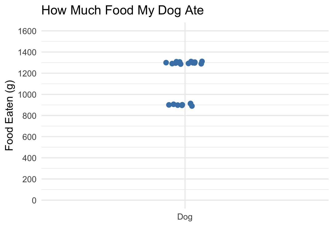
But before we dig into that, let’s talk about how much food my dog eats. Each point represents total grams eaten in a day.

If this plot is confusing you, you are asking the right questions. There are clearly 3 separate clouds of data. My thinly veiled trick was that I included all 3 of my dogs in this plot. Here it is again with them separated.

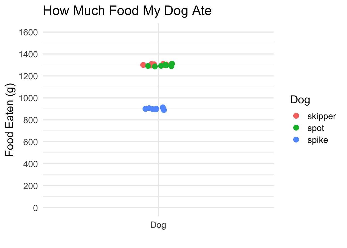
That plot makes more sense! Clearly 2 dogs eat a similar amount of food and 1 eats much less. If this was truly 1 dog, you would expect a plot more like this:

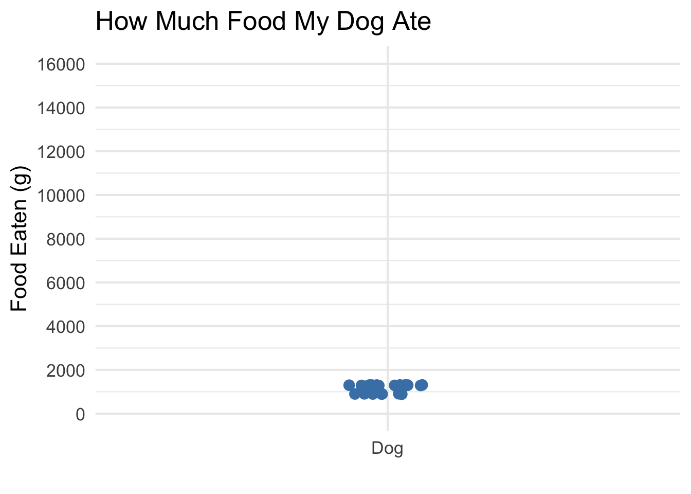
Oops! More trickery. That is actually the exact same “3-dog data” again, only this time the y-axis has been adjusted. But that does uncover one important principle: scaling plays a big part in determining whether or not groups are considered different. (The first and third plots are the exact same data except for the scaling, yet the difference in groups is obvious in one and hidden in the other.)

Let me demonstrate another principle: that of variance.

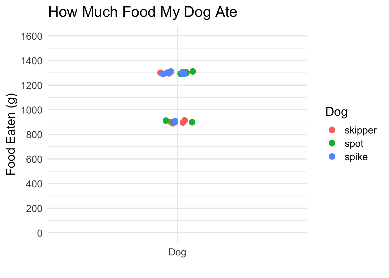
That plot might be the most confusing yet. Can you still draw the conclusion we made earlier: “2 dogs eat a similar amount of food and 1 eats much less”? It is actually — yet again — the same data, but in different groupings. Those different groupings make the result absolutely inconclusive. Why? Because the range of values within a single dog is now so large that it’s hard to tell what’s just normal range and what’s an actual difference between dogs.

Let’s summarize what we’ve learned so far. When comparing means, we need to consider 2 things:

The scale
The variance

So far, we haven’t actually looked at the means at all. And if you stick around a little longer, we’ll reveal why that’s not even necessary.

Let’s run the ANOVA test you may be familiar with, but confused by.


Call:
lm(formula = grams ~ dog, data = long_data_mixedUp)

Residuals:
   Min     1Q Median     3Q    Max 
-302.4 -206.5  101.1  149.8  207.0 

Coefficients:
            Estimate Std. Error t value Pr(>|t|)    
(Intercept)  1101.00      71.43  15.414 6.36e-13 ***
dogspot        50.75     101.01   0.502    0.621    
dogspike       99.37     101.01   0.984    0.336    
---
Signif. codes:  0 '***' 0.001 '**' 0.01 '*' 0.05 '.' 0.1 ' ' 1

Residual standard error: 202 on 21 degrees of freedom
Multiple R-squared:  0.04406,   Adjusted R-squared:  -0.04698 
F-statistic: 0.484 on 2 and 21 DF,  p-value: 0.623

Note that this is the last version of the data, where each dog’s eating varied widely. And sure enough, the data does not reveal any dog as different. If you’re unfamiliar with this output in R, just look at the right-most number on the last row, labeled p-value. It reads .623. This means that if there truly were no difference between dogs, we would see a difference this large (or larger) about 62% of the time, just by random chance. If that’s still confusing, don’t fret. We’ll come back to it. Let’s take a detour into some of the other numbers here.

Starting with the Estimate column: this is a measure of how much a group differs from the reference group. In this case, our reference dog is Skipper (the output doesn’t say that explicitly, but since I know there are 3 dogs — Skipper, Spot, and Spike — and Skipper is missing from the output, that tells me it’s the reference). Spot’s estimate is 50.75 and Spike’s is 99.37. That means Spot is estimated to eat 50.75 more grams than the reference dog, and Spike is estimated to eat 99.37 more grams than the reference dog. So, done, right? There’s a difference: they both eat more than Skipper. Why does the model’s p-value say “no way there’s a difference”?

Remember the second problem we uncovered: variation. For this, we look at the column for Std. Error, or standard error. This is a measurement of how uncertain we are about the mean. For now, just think of it as similar to the standard deviation (it isn’t exactly, but it’s related — stay tuned for a different post that explains the difference). The standard error, for now, can be thought of as how much we expect the data to vary. In this case, Spot and Spike share a standard error of 101.01 (Shared? Yes — just accept that for now). In other words, just from natural variation, we can easily expect +/- 101 grams of variation. Their consumption of 50.75 and 99.37 more grams of food falls well within the range of “random variation we’d expect.” So the data suggests that 50.75 and 99.37 could just be the result of natural variation.

And now, working backward to the first principle: scaling. If I told you this was measured in grams, or kilograms, or even something nonsensical like pounds, you should expect the same conclusion: the dogs do not appear to eat different amounts. The calculation of Estimate and Std. Error is done independent of the units of scale. It controls for scale rather than be fooled by scale.

The test concludes the following: “based on how much variation I see in your data, there’s too much randomness to think any of these dogs is different.”

You might ask, “What if the dogs are completely separated but still highly variable?” Like we learned before, that alone is a scaling issue. Zoom out far enough and they could look the same. What we want is a test that bakes the consideration of scale into its methodology, and that’s what ANOVA does.

“How little variation would need to be present to conclude this is a single population?”

Notice, nothing about means. Differences in means can be made to look bigger or smaller just by zooming in and zooming out.

Let’s close the loop. Let’s look at the original data, where 1 dog is clearly separate from the other 2.


Call:
lm(formula = grams ~ dog, data = long_data)

Residuals:
    Min      1Q  Median      3Q     Max 
-12.125  -4.969  -1.000   4.844  14.750 

Coefficients:
            Estimate Std. Error  t value Pr(>|t|)    
(Intercept) 1302.875      2.597  501.643   <2e-16 ***
dogspot       -6.625      3.673   -1.804   0.0856 .  
dogspike    -400.750      3.673 -109.106   <2e-16 ***
---
Signif. codes:  0 '***' 0.001 '**' 0.01 '*' 0.05 '.' 0.1 ' ' 1

Residual standard error: 7.346 on 21 degrees of freedom
Multiple R-squared:  0.9987,    Adjusted R-squared:  0.9985 
F-statistic:  7807 on 2 and 21 DF,  p-value: < 2.2e-16

p-value: .0000000000000022. Oh yeah - there’s something different here. Spot eats 6.625 fewer grams than Skipper. But look at Spike! Spike eats 400.750 grams fewer! Is that a lot? You better believe it. We’d reasonably expect variation of only 3.673 grams! That Estimate is 109 times greater than the Std. Error. (How did I calculate that so fast? That’s exactly what the t-value is: how much greater our estimated effect is than the variation we’d reasonably expect.)

Again, nothing about means.

Question: Why do we use Analysis of Variance (ANOVA) to compare means? Answer: Raw mean differences, on their own, don’t tell us much — they can be hidden or exaggerated by scale, and they can be swamped by natural variation. ANOVA compares the differences between group means to the variation we’d expect within groups, which is why it’s built on variance rather than means alone.